We continue to assume that LWS is topically organised, that is to say, for example, that the parts of the LWS carrying visual information will include structures which echo, in a simple way, the real world structures to which they refer.
This note is by way of a tutorial example: how we might represent a three dimensional surface by a two dimensional graph or network. Or put another way, how do we represent three dimensional solids in our two dimensional patch of cortex, a representation which has come through the two dimensional retinas? Inter alia, part of a drive to get to know a bit more about the workings of graphs, which may well inform those of networks.
Our example
Let us suppose that we have a well behaved, two dimensional, continuous surface S embedded in three dimensional space, a surface which encloses a finite, three dimensional, convex object.
 |
| Figure 1 |
Our origin is roughly in the middle of this object.
We imagine the surface of a sphere, centred on that origin and a family of lines and planes through that origin, dividing up the surface of the sphere into a large number of spherical versions of equilateral triangles, all exactly the same size and shape. Colour aside, a small portion of the surface of our sphere is approximated by the left hand diagram of Figure 1 above.
We now consider the triangulation of our surface S induced by projection of this same family of lines and planes onto it (the triangular projection). A triangulation which can be represented as a special sort of graph G. A graph in which exactly six edges meet at every point, that is to say vertex, in which every face has three sides, that is to say edges, and which satisfies Euler’s rule that V-E+F=2, that is to say vertices minus edges plus faces (aka regions, in this case triangles) equals two.
We suppose that this triangulation is fine enough that it yields a satisfactory approximation to the surface so triangulated. An approximation which is helped along by the assumptions of continuity and convexity.
We now project G onto a disc in the plane, say a parallel projection (the parallel projection), the results of which are rather crudely approximated by the right hand diagram of Figure 1, but hopefully it gives the idea, in particular the bunching around the perimeter. We call the projected version of G, P(G).
We can express P(G) using the neurons of our (approximately) two dimensional sheet of neurons. We suppose that the synapses expressing the connections are all of equal strength, in some sense or another – but clearly the connections are not all going to be of equal length. The action potential transmission times, while small, are not going to be equal, and in this connection, as an aside, we offer some numbers:
- Our patch of cortex is about one centimetre square
- There might be 100,000 neurons to the square millimetre
- Action potentials might travel at 100 metres/second
- Action potentials might last one millisecond
- During that time they might travel 10 centimetres.
 |
| Figure 2 |
P(G) is a directed graph and we suppose that the source of this graph is the red spot on the right hand diagram of Figure 1. Activation then flows down and around our surface, ending up at a sink around the back, unseen on this diagram. So we know that the red spot is on the front of our surface S, from our present point of view.
The first idea
P(G) is going to get a bit bunched around the perimeter. We might allow a small amount of head movement, small changes in the point of view to resolve that bunching. In any event, we suppose that G has been faithfully projected onto the neurons of P(G).
Maybe the fact that we have two retinas, a short distance apart from each other, helps. Maybe that more or less does the trick, leaving very little residual need for movement.
The second idea
P(G) will have lots of crossing lines because the front of S has been superimposed on the back. Crossings which will confuse our reconstruction of S. However, graph theory will tell us that P(G) can be mapped in a sensible way onto the surface of a sphere, or, indeed, any other surface of the same sort. A mapping which will give us a nice triangulation of the surface of that sphere with no crossing lines. With no need for tori or other more complicated objects to resolve crossings. No crossing-resolving bridges like the handles of teacups.
We call the plane containing P(G) the reference plane.
The idea is then that we can reconstruct our surface S from the shape of the triangles of P(G), that we can compute the angle which the target triangles of G triangles makes with the reference plane and that we can rebuild our surface, triangle by triangle, working out from the source, the source marked by the red spot.
But do we really have enough information in P(G) to do this? Is our solution going to be unique?
 |
| Figure 3 |
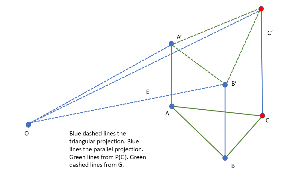
Given the parallel projection, we know that C’ lies on the line C’C.
Given a triangular projection, the angles between adjacent lines of projection must all be the same, so if we have OA’ and OB’, we can also work out where OC’ is. We don’t even need to know what the angle is; the fact that they are all the same suffices.
Noting here that there are actually two possibilities for OC’, one above and one below the plane defined by the triangle OA’B’, corresponding to the two triangles in which each edge participates.
We assume that, given our orderly progress around our orderly surface S, that it is always clear which of these two possibilities is the solution. Allowing that there may be some little local difficulties.
And C’ is the point of intersection of CC’ and OC’. So we can recover the position of C’.
And so working through our triangulation, we can recover the surface S from P(G).
Given that this process springs from an edge rather than a vertex, we might need to assume that at the source, at our red spot, the surface is orthogonal to the point of view. That we have one small patch of triangles which really do look equilateral, one small patch which can get us started.
 |
| Figure 4 |
Conclusions
We do not claim that the machinery we have exhibited above is the way that neurons do things. Indeed, it seems much more likely that they use subtle changes of colour to do much of the work we have given here to triangulations.
But we do claim that this example illustrates how the interplay of prior knowledge – the triangular projection onto a well behaved convex surface – with incomplete sensory information – the projection P(G) – can be used to reconstruct the object – the well behaved convex surface S – being sensed.
It would be interesting, using the sort of machinery deployed at reference 2, to model the stimulation of a network of neurons modelling or expressing P(G). To find out whether the activation signature of one surface differed in some organised way from that of some other surface. Or from that from some other point of view. But that will have to be left to others.
PS: google image search does the business on this occasion, getting from the version available at reference 3 to the original version of the very same picture included above as Figure 4. No idea now why I thought it necessary to use the MS snipping tool at reference 3, rather than just loading up the original picture.
References
Reference 1: http://psmv3.blogspot.co.uk/2017/08/big-brains.html.
Reference 2: Cliques of Neurons Bound into Cavities Provide a Missing Link between Structure and Function – Michael W. Reimann, Henry Markram and others – 2017. One of the references to be found at reference 1.
Reference 3: http://psmv3.blogspot.co.uk/2016/10/meeting-in-middle.html.
Group search key: srd.
No comments:
Post a Comment